Theo Jansen Matlab Simulation

My roommate had to do a simulation of a Jansen mechanism for his kinematics class. It sounded interesting so I gave it a try. Here is what I came up with:







Doing a simulation of a mechanical linkage was something I had never done, nor even really thought about. I initially tried to express all the angles as functions of each other but this soon became insane (this could very well be due to the fact that I am in Electrical Engineering and have never taken a kinematics course before so I had no idea what the proper equations would even look like). After trying to simplify gigantic trig equations in wolframalpha.com and getting back stuff that was disgustingly crazy I resorted to my middle school way of solving equations I don't really understand: brute force. (I used to make programs on my TI-83 to brute force single (and even double) variable equations way back in the day)

So there was only three things I really had values for: the length of the legs, the distance between the crank and the pivot, and the angle of the crank. So say the crank is at a certain angle and you know its length, you can find the end point x,y using simple sin and cos. Now the end of the crank (node 0) needs to be connected to node 1. Node 1 is a known length off the pivot, link_9. So basically what I do is rotate link_9 around the pivot until the distance between node 1 and node 0 are extremely close to the length of link_1. I find this really hard to explain still even after trying to do it many times. Basically I brute force the angle of a bar until the tip of the bar is a certain length away from the other bar it needs to connect to (the distance which I know, since I know the length of all the legs).

Even though this method is absolutely confusing to explain in words it is extremely modular and dead simple to implement. The code is basically the same thing over and over again just with different bars and also some angle constraints (you know link_9 will always be between 45 and 135, roughly). Adding new bars is as simple as copy and pasting and changing the names of the variables. I can literally make any mechanism this way without doing a single line of hard coded trig.

I found the paper linked below to be extremely helpful for providing good bar lengths. All the nodes and bars in my code are named the same as those in this paper
http://ujdigispace.uj.ac.za:8080/dspace/bitstream/10210/1738/39/Numerical.pdf

Edit: For some reason the link does not work, to find the paper google: "Numerical kinematic and kinetic analysis of a new class of twelve bar linkage for walking machines"

%Max Thrun
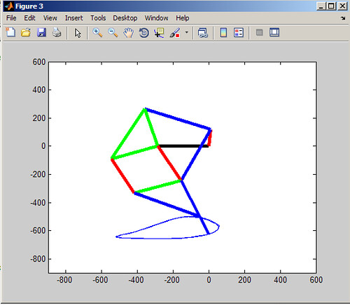
%Simulation of Jensen Mechanism

close all               %Clsoes windows
clear all               %Clears all variables
clc                     %Clear command window

%Declare variables

crank_r = 120;
link_1 = 400;
link_2 = 389;%400;
link_3 = 275;
link_4 = 400;
link_5 = 275;
link_6 = 400;
link_7 = 275;
link_8 = 275;
link_9 = 275;
link_10 = 275;
link_11 = 412;%540;

crank_x = 0;
crank_y = 0;

pin_x = crank_x - (286/1);
pin_y = crank_y;

node_1_x = pin_x;
node_1_y = 5;

link_9_t = 0;

link_10_t = pi;
link_11_t = pi;

node_2_x = pin_x - link_9;
node_2_y = pin_y;

link_8_t = 3/4*pi;

node_3_x = pin_x;
node_3_y = pin_y - link_8;

link_7_t = pi;

node_4_x = pin_x - link_7;
node_4_y = pin_y - link_3;

link_5_t = 3/4*pi;

node_5_y = pin_y - link_8 - link_5;
node_5_x = pin_x;

node_6_y = node_5_y;
node_6_x = node_5_x;

axis([-300 300 -300 300]);
grid on                 %Display grid on plot
xlabel('real axis');    %Give the xlabel
ylabel('imag axis');    %Give the ylabel
title('Example 1');     %Give the title of the plot


avi = moviein((8*pi+pi/2)*5);

%Animation
figure(3)

i=0;

x = [];
y = [];

for t=0:0.1:8*pi+pi/2+pi;

    i = i + 1;

    node_0_x = crank_x + crank_r*cos(t);
    node_0_y = crank_y + crank_r*sin(t);

    
    %
    % NODE 1
    %

    dist = 10000000;
    
    for link_9_t=0:0.02:pi;
        node_1_x = pin_x + link_9*cos(link_9_t);
        node_1_y = pin_y + link_9*sin(link_9_t);

        dist_tmp = sqrt((node_0_x-node_1_x)^2+(node_0_y-node_1_y)^2);

        diff = abs(dist_tmp - link_1);

        if (diff < dist)
            dist = diff;
            theta = link_9_t;
            %fprintf('New theta: %d  Diff: %d\n', theta, diff);
        end
    end
    
    link_9_t = theta;
    
    node_1_x = pin_x + link_9*cos(link_9_t);
    node_1_y = pin_y + link_9*sin(link_9_t);
    
    
    %
    % NODE 2
    %
    
    dist = 10000000;
    
    for link_10_t=.75*pi:0.02:1.5*pi;
        node_2_x = pin_x + link_10*cos(link_10_t);
        node_2_y = pin_y + link_10*sin(link_10_t);
    
        dist_tmp = sqrt((node_2_x-node_1_x)^2+(node_2_y-node_1_y)^2);
        
        diff = abs(dist_tmp - link_2);
        
        if (diff < dist)
            dist = diff;
            theta = link_10_t;
            %fprintf('New theta: %d  Diff: %d\n', theta, diff);
        end
    end
    
    link_10_t = theta;
    
    node_2_x = pin_x + link_10*cos(link_10_t);
    node_2_y = pin_y + link_10*sin(link_10_t);
    
    %
    % NODE 3
    %
    
     dist = 10000000;
    
    for link_8_t=pi:0.02:2*pi;
        node_3_x = pin_x + link_8*cos(link_8_t);
        node_3_y = pin_y + link_8*sin(link_8_t);
    
        dist_tmp = sqrt((node_0_x-node_3_x)^2+(node_0_y-node_3_y)^2);
        
        diff = abs(dist_tmp - link_6);
        
        if (diff < dist)
            dist = diff;
            theta = link_8_t;
        end
    end
    
    link_8_t = theta;
    
    node_3_x = pin_x + link_8*cos(link_8_t);
    node_3_y = pin_y + link_8*sin(link_8_t);
    
    %
    % NODE 4
    %
    
    dist = 10000000;
    
    for link_7_t=.75*pi:0.02:1.5*pi;
        node_4_x = node_3_x + link_7*cos(link_7_t);
        node_4_y = node_3_y + link_7*sin(link_7_t);
    
        dist_tmp = sqrt((node_4_x-node_2_x)^2+(node_4_y-node_2_y)^2);
        
        diff = abs(dist_tmp - link_3);
        
        if (diff < dist)
            dist = diff;
            theta = link_7_t;
        end
    end
    
    link_7_t = theta;
    
    node_4_x = node_3_x + link_7*cos(link_7_t);
    node_4_y = node_3_y + link_7*sin(link_7_t);
    
    
    %
    % NODE 5
    %
    
    dist = 10000000;
    
    for link_5_t=pi:0.02:2*pi;
        node_5_x = node_3_x + link_5*cos(link_5_t);
        node_5_y = node_3_y + link_5*sin(link_5_t);
    
        dist_tmp = sqrt((node_4_x-node_5_x)^2+(node_4_y-node_5_y)^2);
       
        diff = abs(dist_tmp - link_4);
      
        if (diff < dist)
            dist = diff;
            theta = link_5_t;
            %fprintf('New theta: %d  Diff: %d\n', theta, diff);
        end
    end

    link_5_t = theta;

    node_5_x = node_3_x + link_5*cos(link_5_t);
    node_5_y = node_3_y + link_5*sin(link_5_t);

    node_6_x = node_3_x + link_11*cos(link_5_t);
    node_6_y = node_3_y + link_11*sin(link_5_t);

    x(end+1) = node_6_x;
    y(end+1) = node_6_y;

    %
    % DRAW
    %

    plot([crank_x pin_x], [crank_y pin_y],'black','linewidth',4); hold on       % crank to pin
    plot([crank_x node_0_x], [crank_y node_0_y],'r','linewidth',4); hold on     % crank

    plot([node_0_x node_1_x], [node_0_y node_1_y],'b','linewidth',4);           % link_1
    plot([pin_x node_1_x], [pin_y node_1_y],'g','linewidth',4);                 % link_9

    plot([pin_x node_2_x], [pin_y node_2_y],'g','linewidth', 4);                % link_10
    plot([node_1_x node_2_x], [node_1_y node_2_y],'g','linewidth', 4);          % link_2

    plot([node_0_x node_3_x], [node_0_y node_3_y],'b','linewidth',4);           % link_6
    plot([pin_x node_3_x], [pin_y node_3_y],'r','linewidth',4);                 % link_8

    plot([node_3_x node_4_x], [node_3_y node_4_y],'g','linewidth', 4);          % link_7
    plot([node_2_x node_4_x], [node_2_y node_4_y],'r','linewidth', 4);          % link_3

    plot([node_3_x node_5_x], [node_3_y node_5_y],'r','linewidth', 4);          % link_5
    plot([node_4_x node_5_x], [node_4_y node_5_y],'b','linewidth', 4);          % link_4

    plot([node_3_x node_6_x], [node_3_y node_6_y],'b','linewidth', 4);          % link_5

    plot(x,y);

    hold off            %So next plot will erase the current plot
    axis([-900 600 -900 600]);
    %pause(0.001)          %Stop execution for 0.1 sec so that the animation can be seen
    avi(i) = getframe(gca);
end



movie2avi(avi,'jansen.avi','compression','cinepak') % or cinepak, indeo5